ANCOM explained

In case you have not heard, ANCOM is another differential abundance test, designed specifically for tweezing out differentially abundance bacteria between groups.  Now, note that there are a ton of differential abundance techniques out there.  And one might ask why are there so many people focused on this seemingly simple problem.

It turns out that this problem is actually impossible.   And this is rooted into the issue of relative abundances.  A change of 1 species between samples can be also explained by the change of all of the other species between samples.   Let's take a look at simple, concrete example.

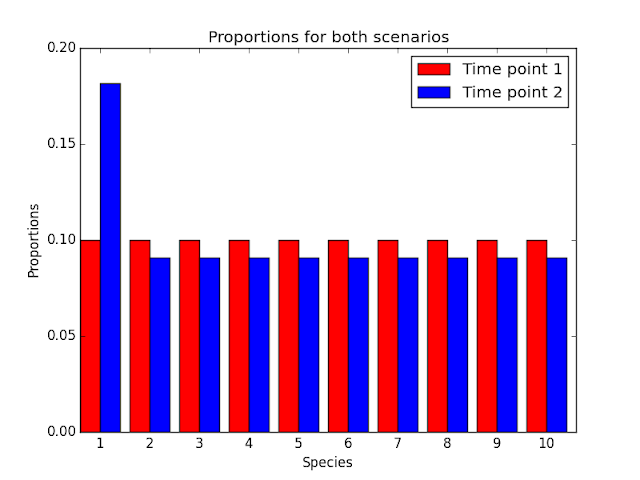
Here we have ten species, and 1 species doubles after the first time point.  If we know the original abundances of this species, it's pretty clear that species 1 doubled.  However, if we can only obtain the proportions of species within the environment, the message isn't so clear.

Above are the proportions of the species in the exact same environment across the two time points.  Here, it appears that everything is changing, which isn't the case in the original environment.  Also, there are multiple hypotheses that could explain the change of proportions.  For instance, it is a valid hypothesis that species 2-10 all halved.  In fact, there are an infinite number of hypotheses that explain this change of proportions, making the differential abundance problem impossibly difficult.

You cannot hope to solve the differential abundance problem without making some assumptions.  DESeq2 makes assumption using the Negative Binomial distribution.  metagenomeSeq makes the assumption using Zero Inflated Gaussian distribution.

ANCOM does make its own set of assumptions, making it a little differient from the conventional differiential abundance tool. There are two things that makes this tool very strong

It makes no assumption about independence between features. 

When you think about how OTUs are sampled in the first place, this makes sense.  All OTUs are sampled without replacement from some environmental sample.  The sampling process itself imposes dependence between the OTUs.  And this isn't even accounting for all of the ecological dependencies present.   If you'd like some resources to check out statistical sampling, I'd start off checking out the Multinomial distribution.   With this reasoning,  it doesn't really make much sense to apply univariate tests (i.e. t-test, anova mann-whitney) directly on OTU tables to identify differentially abundant species, since they implicitly assume independence between the OTUs.


It makes few assumptions about the distributions of the OTUs.

Due to the highly dependent nature of our data sets, its actually quite difficult to formulate meaningful distributions.  ANCOM's strategy is to run tests on the log ratios across OTUs rather than the OTUs themselves.  There are a few clear cut advantages of using this approach.

1. log-ratios are ideal for detecting large relative changes.  Think about it, the changes in the most abundant OTUs will drown out the changes in the lower abundant OTUs.  An OTU that is present in 0.01% of the reads that then grows to 0.05% of the reads actually increased by 5x fold, which is huge!  But if you only look at percent increase, its just 0.04% which may seem insignificant. 
2. log-ratios are actually ideal for normalizing for sequencing depth.  If you have OTUs $x$ and $y$, with counts $n_x$, $n_y$ in a sample with $n$ reads, then the log ratio will work out to be \[\ln \frac{n_x}{n_y} = \ln \frac{n p_x}{n p_y} = \ln  \frac{p_x}{p_y} \]  where $p_x$ and $p_y$ are the proportions of $x$ and $y$ in the sample.  Note that the sequence depth constant completely disappears.  Now there are still a few issues with resolution, that is a discussion for another time.

In light of these advantages, ANCOM does make a few assumptions.  ANCOM actually assumes that there are few species changing.  In the supplemental materials Assumption A, they do assume that less than $p-2$ species are changing, if there are $p$ species present in the environment.  But looking at Figure 2, there is a drop power when 25% of the species are differentially abundant.  So its not clear exactly how strong this assumption is.  If there are really $p-2$ species changing in the environment, that raises some concerns in my mind.  Would differential abundance be the question that we really care about?  I don't think so.

Another concern that ANCOM raises is the problem of zeros.  You cannot take the log of zero.  This is an active research problem in the compositional data analysis community, making ANCOM no less vulnerable to this issue.  So the more zeros that your dataset has, the less you should be trusting your results.  Now there are a few approaches to this problem.  One approach is to introduce pseudo counts.  In the scikit-bio code, one of the recommended solutions is to use multiplicative_replacement.  An equally valid alternative is to just add a constant, such as 1, to all of your counts.

Another approach is to combine features together.  For instance, when we are looking at OTUs, we can typically infer some phylogenetic tree.  Rather than running the test on the OTU abundances, we could run the test on genera abundances, which often yields less zeros.

Of course, before running ANCOM, you'll want to filter out contaminants and low abundance samples.  These will just add noise to your results.  I typically filter out samples less than 1,000 reads and OTUs that only appear 10 times in the study.  But this is just a rule of thumb that I developed - definitely needs some benchmarking.

So in conclusion, ANCOM is a very powerful tool.  But it does have some issues that you need to watch out for.  (1) Large numbers of changing features and (2) large numbers of zeros.  If you observe a huge number of OTUs that are significantly different (i.e. more than 25% of your OTUs) from ANCOM,  there is a chance your dataset is stretching the limits on ANCOM's assumptions.  Furthermore, if you are running into these issues, then maybe answering the differential abundance question is not fruitful.  You can also try using volcano plots to visualize the ANCOM results, and plot the W-statistic along the y-axis.  Log scaled boxplots also help, but can be overwhelming if there are many significantly differential OTUs.